The purpose of this analysis is to assist the Public Interest Law Center of Philadelfor phia in developing a comparative public health based criteria advancing Environmental Justice. In general we were concerned with the census tract mapping of four health factors in Philadelphia,Pa.(1,500,000 pop., 367 census tracts).

            *   Age-adjusted cancer mortality rate

            *   Age-Adjusted non-cancer mortality rate

            *   Infant mortality rate

            *   Low birth weight rate

    Additionally, the Environmental Background Information Center (EBIC)  was concerned with the spatial analysis of human population data in
Pennsylvania and its relation to the existing sources of environmental stress such as solid waste and hazardous waste treatment nod disposal facilities as well as
manufacturing facilities and coal mining facilities.

    The rationale for the public health study is based on the view that a community that has substantially worse public health than the median (or average) public health  of the population in the other areas of the city or county or state, should not have its poor public health exacerbated by the introduction of a new source of  environmental stressors.

    The public health study, it should be noted, concerns the existing community health regardless of the possible causes of the condition; the study does not examine the environmental conditions or the effects of odors, noise, mobile emissions, psychological conditions or personal habits, or cultural habits, or educational levels, or income levels, or medical facilities, etc., all of which certainly affect individual health and community public health.

    This is not to say that there may not be strong correlations between the public health of a community and one or more of the above noted conditions. The EBIC study was designed  to examine how human health factors were distributed spatially with respect to environmental risks and other demographic features of the
population.

    To undertake this study we used a number of statistical tools to help explore and explain these relationships. in the opening section.   In the opening section, I address this problem at a level of abstraction which is specifically intended to provoke the reader. Immediately this provocation is likely to lead the reader to dismiss the text insofar as it belabors the obvious. However this might arise, the challenge I present here to the reader is to provoke thought which pushes the human condition to a level of abstract consideration which sets aside blame and guilt for purposes of a more general consideration of the circumstances which we all arbitrarily find ourselves in after we are born and become conscious of our material status.
 

Summary of Key Preliminary Findings
 

Our work with numerous datasets made available from state and federal agencies informs us that at the municipal level in PA:
 

• These data indicate that poor health correleates with poverty, low income and low educational attainment.  These factors contribute to a diminished quality of life for many Pennsylvanians.

• Philadelphia, which contains the highest population in the state, and which is both a municipality and a county, has some of the poorest health in the state. The distribution of poor human health outcomes in Philadelphia follows patterns which are apparent at the municipal level.

• Some small municipalities in Pennsylvania are experiencing high rates of poor health, but because of their size, these trends cannot be adequately assessed. The state needs to develop longer term measures to monitor human health in these areas.Environmentally harmful facilities are more likely to be found in communities composed of impoverished minorities and whites. This is true when we control for the size of municipalities both geographically and demographically.

 
• The distribution of social resources follows observable patterns which are statistically significant. Urban areas tend to exhibit high degrees of social segregation between rich and poor, advanced and non advanced education, as well as between minority and non minority. Rural areas tend to be composed of whiter populations with lower educational attainment, lower income levels and higher levels of poverty.

 
• State and federal environmental and census data indicate that there are evident patterns of class and racial inequality in the distribution of environmentally hazardous facilities in Pennsylvania. These facilities include manufacturers releasing toxins to the environment, solid waste handling and disposal, and hazardous waste disposal facilities.

Research on human population distribution is certainly not new. However, research on human population distribution which examines the distribution of social resources is emerging as a relatively new and increasingly sophisticated field. Some research along these lines has shown evidence of racial and class discrimination, for example, in the amount of environmental risk to which human populations are exposed. Environmental risk constitutes a form of negative social resource which, in some research, has come to serve as an indicator of broader social discrimination. In our view, this type of research represents an advance in our current means of understanding the social structure which we all inhabit. While it is far from a perfect research regime, it offers considerable insight into the manner in which we perceive, experience and share our own environment in our own communities. In this section, I outline a broad view of the approach to this research project.
 

The relative geographic distribution of different age, class, racial and ethnic sub-populations across space is an institutional dimension of modern society. By institutional, I mean that the circumstances of different groups (racial and class groups in particular) largely exist prior to our own individual existence and perception. Within this context, there is a close relationship between the distribution of human population groups and human activities such as waste handling, manufacturing, and mining. These phenomenon coincide with certain geographic/natural features of land. Features which make - and have made - certain areas more desirable for purposes of human occupation, settlement, and economic activity.
 

Human population distribution is thus the result of a convergence of numerous factors including geologic and historical processes, cultural, familial, and physical proximity and the availability of a livelihood of some sort. Some places are better for human habitation because, for various reasons, they are more habitable. Some places, while not more habitable than others - perhaps even less so - support large populations because of the emergence of significant economic activity related to the flow of goods and commerce - largely as the result of geographic features beneficial to human trade such as transportation infrastructure.
 

At issue in environmental justice research is whether or not such geographically located sub-populations are a) disadvantaged and b) exposed to serious risks from productive human activity for which no net benefits accrue which might otherwise tend to ameliorate the conditions associated with being disadvantaged, and c) caught in those conditions as the result of broader patterns of discrimination stemming from systemic racism. In this analysis, I attempt to discern some of the patterns associated with the hypothesis that class and racial discrimination is apparent in the distribution of poor health and environmental risk.
 

Literature
 

A considerable body of literature has emerged on the topic of environmental justice. Only a small portion of it is empirical and that portion is somewhat varied in its findings. This variation in analytical results can be summarized as arising from different research methodologies (see Lipsett and Mennis, 1999). In particular, these research methodologies vary in their approaches temporally, in scope, and in scale. Temporal variation in analytical results is related to the chicken and egg question: i.e. do disadvantaged groups move into areas where environmental risks already exist or do the risks move into areas where disadvantaged groups already live? Methodologies which approach this question have come up with varied results, but they are relatively rare and many feel the question is, for all intents and purposes, irrelevant. Temporal analyses are largely limited in scope to certain confined geographic areas rather than an entire region or the entire nation. Still other variation in results arise out of methodological variation related to the scale of the analysis. This matter is also referred to as the "resolution problem:" i.e. What is the appropriate geographic unit to which population data should be aggregated for purposes of analysis? Many studies focus on this matter and follow a narrow track, arguing for the appropriateness of one or another geographic unit for purposes of analysis.
 

A different literature addresses the spatial clustering of human health problems, in particular, various types of cancer and their occurrence around sources of pollution (e.g. toxic dump sites, manufacturers, etc). Some studies have established statistically significant relationships between sources of pollution and human health problems, but most studies do not, usually because of relatively small sample sizes. However, a small body of literature has examined such things as respiratory mortality and air quality and found statistically significant relationships. For a number of reasons including lack of resources and a lack of sensitivity in the structure of the data available to us, this analysis does not attempt to establish such relationships. Rather we are simply seeking to identify and characterize communities with substandard health and/or contain environmentally hazardous facilities.
 
 
 
 
 

Data
 

This analysis is derived from data which was obtained from a number of different sources including the Philadelphia Department of Health, the Pennsylvania Department of Public Health, the United States Department of Health and Human Services Center for Health Statistics, the United States Envheironmental Protection Agency, the United States Department of the Census, the Pennsylvania Department of Environmental Protection and others. We obtained statistical health data for four health outcomes in Pennsylvania and Philadelphia; Total Mortality, Cancer Mortality, Infant Mortality, and Low Birth Weight. These data were averaged over five years - 1992 to1996. These statistics were derived from data provided by the Pennsylvania Department of Public Health for each municipality and county in Pennsylvania and the Philadelphia Department of Health for census tracts in Philadelphia. The health data was combined with demographic data from the 1990 U.S. census as well as population projections for 1996, 2001 and 2006 provided by the Environmental Systems Research Institute (ESRI). We also obtained and examined data on manufacturing activity, solid waste and hazardous waste disposal activity, and coal mining activity from the U.S. EPA's TRI, RCRIS, and BRS databases and the Pennsylvania Department of Environmental Protection.
 

Methodology
 

This paper addresses the problem of the spatial distribution of human health, demographic and environmental risk phenomenon through a limited multi-scalar analysis which is confined in scope to the state of Pennsylvania. The overall approach taken here is to utilize three scales of resolution, the county, the municipality, and the census tract. In addition, statewide levels are applied as an additional background standard. It should be noted here however, that health data in Pennsylvania is collected by the state at the municipal level and is coded so that it can be aggregated to the county level. In Pittsburgh and Philadelphia, human health data is also aggregated at the census tract level, allowing for an additional scale of detail for those areas. This "data reality" does have a limiting effect on our analysis, however I believe that the multi-scalar approach taken here mitigates some of the problems noted in the literature, at least somewhat. 
 

Our statistics were standardized to derive rates for respective geographic units; i.e. census tracts, municipalities and counties (note; at this stage this discussion only applies to the state, county and municipal levels and not for Allegheny and Philadelphia County census tracts). Cancer mortality and total mortality data was age adjusted to account for variation in age groups between various municipal levels. The age adjustment standard we utilized is the 1940 standard million. The health data was combined with demographic data from the 1990 U.S. census and we then added data on manufacturing activity and hazardous waste disposal from the U.S. EPA's TRI, RCRIS, and BRS databases. These different datasets were combined through spatial and code specific techniques to generate files which incorporated all relevant data which applied to each of the geographic units in question. 
 

Subsequent to mapping relevant data, we conducted a number of statistical analysis of the data to determine the apparent relationships between the environmental, demographic, and health data characteristics of each spatial unit (i.e. county, municipality, census tract). Because of the data structure and functionality of GIS databases, it is relatively easy to conduct statistical analysis of data for purposes of understanding the relationships between various characteristics of geographic units (counties, municipalities). More advanced statistical techniques also allow the analysis of the spatial relationship of various health and demographic characteristics of and between various geographic units. Because there is considerable variation in the size of the geographic unit in our analysis, the minor civil division, we controlled for the size of the region by including its area and the number of people, families and households in the region in the regression analysis. Our findings are discussed in more detail below.
 

In Philadelphia, we also standardized the data by ranking census tracts in terms of the four health outcomes we acquired from the city (infant mortality, cancer mortality, total mortality and low birth weight rates). In addition, we generated two additional health outcome categories which were useful: non cancer mortality and overall health. 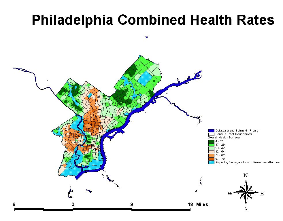Non cancer mortality was derived by subtracting the age adjusted cancer mortality rate from the age adjusted total death rate. Overall health rates were derived by breaking the population into 20 different groups of 5% based on each rate of health outcome. These percentile groups were coded one to twenty with twenty being applied to census tracts with the poorest health for each outcome. I then added the percentile codes for cancer, non cancer, low birth weight rate and infant mortality together and ranking the resulting scores (4 for best combined health to 80 for worst combined health) by the same percentile ranking system (1 - 2O). The overall health variable is useful because it helped to identify areas where people are being hammered with a combination of all poor health outcomes. 
 

The approach taken utilizes several different analytical techniques which are based on Geographic Information Systems as well as statistical and spatial statistical analyses. Age adjustment of the total and cancer mortality rates for each municipality was accomplished with software provided by the Centers for Disease Control. Several different software packages aided us in this analysis including ArcView, ArcView Spatial Analysis Extension, SPSS, Splus, Splus Extension for ArcView, SPlus Spatial Statistics, and Health Information Retrieval System.
 

Findings
 

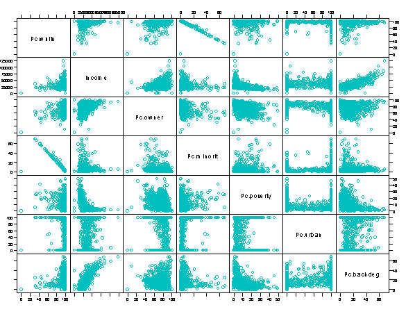
The first section of findings discusses some overall general bivariate relationships apparent in the Pennsylvania data. Each following section discusses a number of complex mulltivariate relationships which help us to get a sense of the structure of the social order in PA and, to a lesser degree, the factors affecting the health of Pennsylvanians in terms of four particular outcomes - infant low birth weight and mortality rates, cancer and total mortality rates. The initial section begins with an overview of the relationships of some of the data in the research model. A number of variables reveal fairly intuitive relationships. Percent Minority and Percent White for example are inversely correlated although not entirely collinear because of variation in the percentages of percent white hispanic between municipalities.

Click on the Graph to see a Larger Version

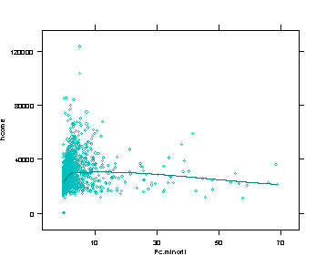
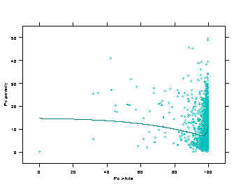
Similar correlations exist between percent bachelor's degree and income. As the percentage of people with a bachelor's degree or higher increases, the median municipal household income increases. As the income level increases, the percentage of people owning homes increases. These more or less intuitive relationships aside, there are other less obvious bivariate relationships which are apparent in the data. For example, as percent minority increases, income levels increase until about 5% minority. The regression line levels out dropping slightly to about 30% minority, which is slightlyhigher than the 24% overall minority level in the United States Census figures from the entire nation. After 33% minority, income levels begin to fall more rapidly. This relationship, not surprisingly, is the mirror image of the relationship between income and percent white, once again illustrating that high poverty rates tend to occur in highly segregated communities more frequently than in integrated ones, although it must be stressed that the very highest income municipalities in Pennsylvania tend to be predominantly white.

In other words, income levels in Pennsylvania are low in certain types of communities which are predominantly white, and other communities which are predominantly minority. This particular reality is best understood in terms of the nature of community structure in Pennsylvania. Impoverished minority populations tend to be clustered in a small number of larger urban municipalities whilst high concentrations of impoverished white people tend to be scattered in rural areas in Pennsylvania. 67.5% of all municipalities in Pennsylvania are classified as 100% rural. 22.8% are classified as 100% urban. The remaining .7% of all municipalities fall somewhere in between those extremes. Thirty-nine municipalities in PA (1.5%) contain populations with greater than 24% minority, the national background figure. 77% of those municipalities are greater than 50% urban. 84 PA municipalities (3.3%) contain minority populations greater than 12%, the state background figure. Once again, 77% of those municipalities are greater than 50% urban.
 

The degree to which this apparent segregation is the result of systematic individual or institutionalized racism probably can never be discerned. But it must be seen as a key factor. To ignore it, or to suggest other explanations for the phenomenon belies the point. Historical processes, geographic features, land use patterns, proximity to transportation routes, all of these may in various ways contribute to the phenomenon, but they do not dismiss the striking evidence of a segregated society, as evinced in 1990 Pennsylvania population data. Having said that, a key point which has been ignored is that racial segregation of communities is one of a number of features of a discernable pattern of broad scale social injustice. 
 

Poverty in rural white communities in Pennsylvania is also marked, and evidence of environmental injustice arises in these communities as well. To emphasize the point, bear in mind that when communities in PA have high percentages of whites, the poverty rate tends to increase sharply, to levels almost (but not quite) as high as those of municipalities with high percentages of minorities. Granted that there are some extremely wealthy, low poverty communities which are predominantly white but they are not the only type of white community and they are not the rule. 
 

Multivariate Analysis

Up till now, of course we've been talking about relationships which are strictly bivariate and do not control for the impact of other factors. These more complex relationships can be better understood using multi-variate techniques a matter to which we now turn. Because there is considerable variation in the size of the geographic unit in our analysis, the minor civil division, we controlled for the size of the region by including its area and the number of people, families and households in the region in the regression analysis. The models and all results, unless otherwise characterized, are statistically significant at the .05 level or greater.
 

Poverty

The relationship between various demographic, and environmental factors and poverty rates in political units in Pennsylvania shows that poverty rates are dependant on a number of factors. Not surprisingly, as median household income levels increase, poverty levels decrease. Educational variables appear in this model to have a counterintuitive effect on poverty rates. As the percentage of people with advanced educations increases, poverty levels increase. Lastly, as the percentage of minority status individuals increases, poverty rates increase. These data do not provide evidence that the presence (or absence) of manufacturing, solid waste and hazardous waste disposal facilities have any relationship with poverty rates at the municipal level. To generalize these results, poverty rates appear to be influenced by a number of factors but not the presence or absence of environmentally hazardous manufacturing and hazardous waste disposal facilities. These findings suggest that the "benefits" of environmentally hazardous facilities and poverty programs do not appear to be reaching many segments of the Pennsylvania population.
 
 
 

Education
 

Educational attainment is often viewed as an important factor in quality of life. Equally, access to advanced education is another aspect of social inequality, with disadvantaged groups having less opportunities for advancement. In this analysis, we found that median household income had a considerable impact on educational attainment. As income increases, educational attainment increases. Curiously, as poverty rates increase, educational attainment also increases but only incrementally. The percent minority and number of environmentally hazardous facilities in a community had small negative effects on educational attainment. Home ownership and percent rural all had negative impacts on educational attainment. These results are somewhat counterintuitive but seem to point to the importance of rural vs urban population settings and economic inequality as defining features regulating educational attainment.
 

Race
 

Minority status is treated as a dependent variable here in order to determine what factors are bound up with that community feature at the municipal level. These results tell us that as the percentages of homeowners increases, the percentage of minority people in the municipality decreases. As the median household income goes up, the percentage of minority people increases. This is also true for poverty rates. As poverty rates increase, percent minority increases. Once again, these results point to disparities in the structure of municipalities with higher percentages of minorities and also clearly points out the fact that most rural municipalities in the state tend to have high percentages of whites.
 

Presence of Manufacturing Facilities and their Releases
 

The presence of manufacturing facilities poses a risk to communities when those facilities are known to handle and release toxic chemicals. The magnitude of the risk to the community, while the subject of an unrelenting debate, is not simply the presence of a given facility in a community, nor the relative proximity of human populations to such facilities. But also to the magnitude of the releases, their relative toxicity, the medium to which they are released and the proximity of people to potential contact with the release either directly or in diluted form. Facilities releasing a class of over 650 chemicals in amounts greater than 25,000 pounds are required to report those releases to the federal government through SARA Title III of the Superfund or CERCLA law. In this analysis we utilized TRI data reported for 1995 to test for the relationship between this source of pollution and the composition of communities containing them.
 

Our results indicate that, in terms of the number of manufacturing facilities present in a municipality, as the percentages of home ownership and percentage of people with bachelors degrees goes up, the number of TRI facilities goes down. Conversely, as the percentage of minority residents and the percent urban increased, the number of TRI facilities increases. In terms of total releases to the environment, a variable which is dependant on the number of manufacturing facilities in an area, as the percentage minority increases, the level of emissions into the environment also increases. These results indicate that manufacturing facilities in Pennsylvania are typically clustered in communities with high percentages of minorities who may be exposed to the emissions from manufacturing activity. It also indicates that communities with larger numbers of manufacturing facilities have lower educational attainment and home ownership rates.
 

Presence of Waste Disposal Facilities
 

TSDF facilities are facilities which hold permits from the U.S. Environmental Protection Agency to handle, treat, store and/or dispose of hazardous waste. Commercial TSDF's constitute a smaller class of these facilities which are licensed to handle wastes and take them in from other non-related business entities for a fee. Several studies have shown that commercial TSDF facilities are most often located in certain areas (zip code regions and census tracts) with higher percentages of minorities than other non-TSDF containing areas (CRJ 1987, 1994, Been, 199x). One set of studies have disputed this relationship but only by eliminating from the analysis all the populations in all census tracts in non-TSDF containing MSA's and rural counties. Our research utilized data provided by Been for commercial TSDF facilities. For a number of reasons, we felt that such a list represented an incomplete inventory of waste disposal activities so we added solid waste disposal facilities including sewage treatment, solid waste transfer stations, landfills, and trash incinerators, provided by the state of Pennsylvania to our analysis. We found that municipalities with higher percentages of minority persons, and persons living in poverty had larger numbers of waste disposal operations. Conversely, communities with higher percentages of home ownership had fewer waste disposal facilities. 
 

Presence of Manufacturing and Waste Disposal Facilities
 

We further profiled the structure of communities to determine what demographic characteristics determined increased numbers of combined waste disposal and manufacturing sources of environmental risk. Educational attainment, home ownership, and percent rural had negative impacts on the total number of environmentally hazardous facilities in Pennsylvania municipalities. Income and minority status have linearly positive relationships with the number of environmentally hazardous facilities. Although the mechanisms behind these former relationships are unclear, it is suggested here that, once again, these findings are an indication of operative disparities in municipalities with larger numbers of environmentally hazardous facilities.
 
 
 

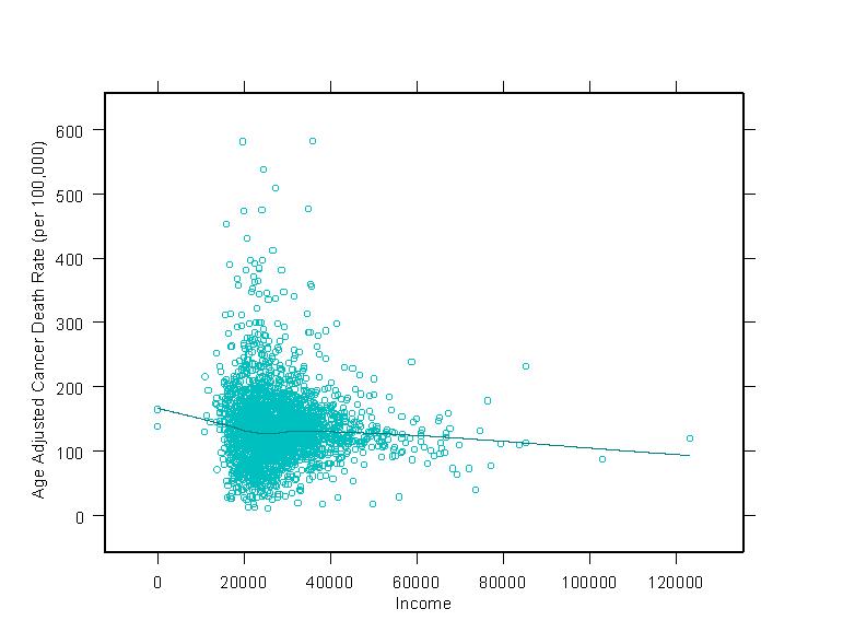
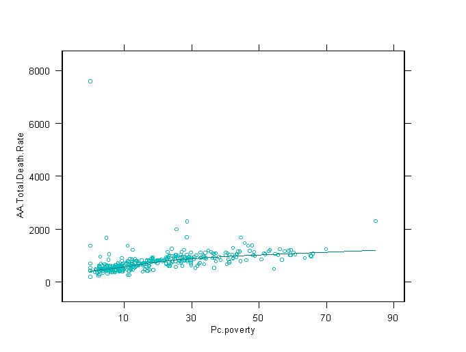
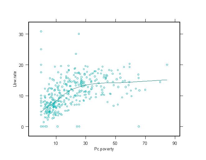
Human Health Outcomes

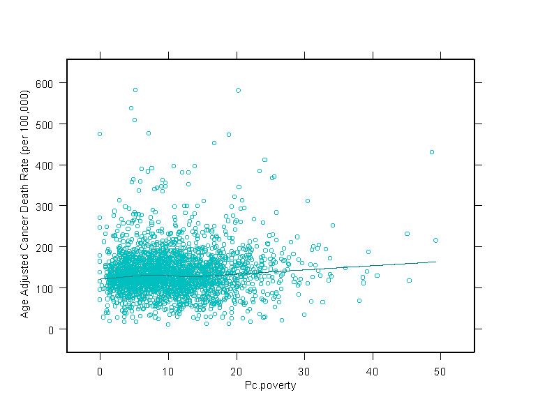
Health wise, there are some observable relationships that bear scrutiny. Poverty and other indicators of diminished economic standing have long been associated with poor health outcomes. This relationship is observable in these data. Age Adjusted Cancer Mortality Rates, Age Adjusted Total Mortality Rates, Low Birth Weight Rates, and Infant Mortality Rates are positively related to poverty rates. As the percentage of people in municipalities living in poverty goes up, rates for these health outcomes also go up. Poor people are, across the board, are more likely to die earlier than people in better economic conditions. Income is, not surprisingly, inversely related to these negative health outcomes. As median household income goes up, mortality and low birth weight rates tend to go down. Some of these relationships are illustrated in the graphs at right. In general economic variables tend to have a positive relationship with health outcomes. As people become more prosperous, their health gets better. Overall, national research indicates that these economic variables drive human health and these findings are supported in our

results in Pennsylvania. Multivariate techniques such as those we use below are a bit less powerful than those above involving demographics, manufacturing and waste disposal. However, there do provide some insight that we discuss below.
 
 

Total Mortality
 

Total Age Adjusted Mortality figures were derived from state municipal health data for the years 1992-1996 and standardized. 1990 ages for 18 age categories were utilized to age adjust raw rates. The age adjusted figures were then plugged into a regression model to derive statistical analysis of the demographic factors affecting the health outcome. Our analysis tells us that home ownership and educational attainment were negatively related to age adjusted total mortality rates. Minority status, percent rural, and percent poverty were all positively related to total mortality. These relationships speak to potential impacts that are occurring within inner city and rural areas and impacting on poor people, leading to elevated total mortality rates.
 

Cancer Mortality

In this model only two variables appear to have any significant relationship to age adjusted cancer mortality; home ownership and educational attainment. Both those relationships are negative. This model is relatively weak insofar as it only accounts for about 3.5% of the variation in the dependant variable. 
 

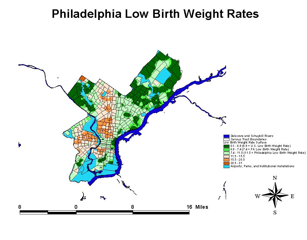
Low Birth Weight

In this model percent minority is the only variable with a significant relationship to low birth weight rates. This relationship is positive. Income is negatively related to low birth weight rates. A considerable body of research involving elevated low birth weight rates for minority populations has linked those outcomes to a lack of prenatal care - a phenomenon which should also be correlated with high poverty and/or low income sot his analysis, to some extent, conforms to broader national level and regional research projects.
 

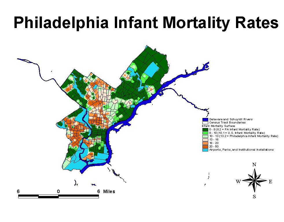
Infant Mortality

No statistically significant relationships were discovered between any of the independent variables discussed above and infant mortality. However, a considerable body of literature on this topic has linked infant mortality to poverty and low income status.

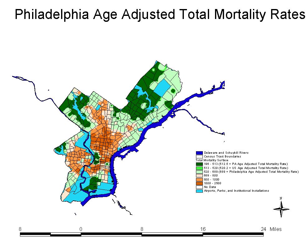
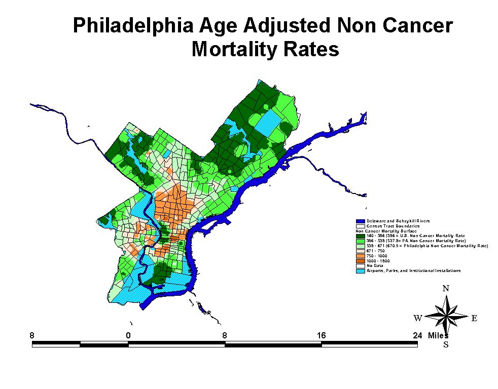
Health in Philadelphia Census Tracts

Philadelphia is not a very healthy city with some of the highest rates of infant mortality, total mortality, cancer mortality and low birth weight babies in the entire state. Not surprisingly, within the city itself, there are even higher rates than the overall citywide rate. This can be shown to be true because the city of Philadelphia collects health outcome data at the census tract level.
 

Analysis of health and demographic data at the census tract level in Philadelphia yields interesting bivariate results, but multi-variate regression techniques utilizing the same basic model as used above, do not appear to be very helpful. The reasons for this are unclear but may be due to outlying data. However, the failure of the regression model to convey explanatory power at multiple scales of geographic aggregation does not undercut the descriptive power of the readily apparent bivariate relationships in the data. Here it should be noted that the overall health of Philadelphia is poor, with poor health outcomes at elevated levels compared to county and municipal averages. The census tract data indicate quite clearly that the distribution of poor health in Philadelphia is not uniform, conforming to the results of the above analysis. In short, some areas of Philadelphia are experiencing poor health at a level which is far above 
most municipalities in the state. As it turns out, those areas with poor health also have elevated levels of poverty, lower incomes and more minorities. Conversely, census tracts with good overall health are predominantly white, have higher incomes, and lower poverty.
 
 
 

Descriptive statistics say much in this regard. By breaking the population down into 20 roughly equal groups, it can be shown that within the 20% of the Philadelphia population with the highest rates of poor overall health in terms of high rates of low birth weight babies, infant mortality, non-cancer and cancer mortality, 94.8% are minorities, 33.4% are living in poverty. This 20% of the population has an average household income of $23,230 per year. Of the 20% of the Philadelphia Population with the lowest rates for these health indicators, 8.1% are minority, 7.4% are living in poverty. The average household income for this group is $41,790 per year.

These same relationships hold true, although in slightly lower magnitude in some cases, for all of the other variables. Here it should be noted that Philadelphia is the most densely populated county and city in the state and so it is something of an anomaly. However, a substantial portion of the state's population is affected by these rates.
 

DiscussionThe core health problems affecting residents of the state are correlated in these data to low income, poverty, and low educational attainment. 

Poverty
 

Coefficients
 

		Unstandardized Coefficients		Standardized Coefficients	t	Sig.
Model		B	Std. Error	Beta
1	(Constant)	25.512	.784		32.547	.000
	PERSONS	1.039E-03	.000	5.129	7.608	.000
	FAMILIES	-2.753E-03	.000	-3.253	-6.534	.000
	HOUSEHOLDS	-1.005E-03	.000	-1.897	-3.402	.001
	AREALAND	2.165E-02	.006	.062	3.642	.000
	INCOME	-5.122E-04	.000	-.723	-27.580	.000
	PC_OWNER	-3.948E-02	.012	-.068	-3.361	.001
	PC_MINORIT	.166	.019	.138	8.508	.000
	PC_RURAL	7.492E-03	.003	.049	2.471	.014
	TOTAL_NUMB	5.326E-02	.100	.013	.534	.593
	PC_BACHDEG	.114	.018	.155	6.168	.000

a Dependent Variable: PC_POVERTY Variables Above the double line are controls
 

Model Summary
 

Model	R	R Square	Adjusted R Square	Std. Error of the Estimate
1	.679	.461	.459	4.874

 

ANOVA
 

Model		Sum of Squares	df	Mean Square	F	Sig.
1	Regression	52314.337	10	5231.434	220.261	.000
	Residual	61064.105	2571	23.751
	Total	113378.443	2581

 
 
 
 
 
 
 
 
 
 
 
 
 
 
 
 
 
 
 
 
 
 
 

Education
 
 
 

Coefficients
 

		Unstandardized Coefficients		Standardized Coefficients	t	Sig.
Model		B	Std. Error	Beta
	(Constant)	1.990	.989		2.012	.044
	PERSONS	-6.967E-04	.000	-2.520	-4.768	.000
	FAMILIES	5.500E-04	.000	.476	1.218	.223
	HOUSEHOLDS	1.520E-03	.000	2.103	4.853	.000
	AREALAND	3.753E-03	.006	.008	.592	.554
	INCOME	8.262E-04	.000	.854	53.377	.000
	PC_OWNER	-.154	.012	-.194	-12.657	.000
	PC_MINORIT	-7.567E-02	.021	-.046	-3.610	.000
	PC_POVERTY	.128	.021	.094	6.168	.000
	PC_RURAL	-3.261E-02	.003	-.156	-10.310	.000
	TOTAL_NUMB	-.326	.106	-.058	-3.075	.002

a Dependent Variable: PC_BACHDEG Variables Above the double line are controls
 

Model Summary
 

Model	R	R Square	Adjusted R Square	Std. Error of the Estimate
1	.821	.673	.672	5.181

 

ANOVA
 

Model		Sum of Squares	df	Mean Square	F	Sig.
1	Regression	142268.529	10	14226.853	529.995	.000
	Residual	69014.281	2571	26.843
	Total	211282.810	2581

 

Race
 
 
 
 
 

Coefficients
 

		Unstandardized Coefficients		Standardized Coefficients	t	Sig.
Model		B	Std. Error	Beta
1	(Constant)	6.850	.919		7.451	.000
	PERSONS	3.303E-04	.000	1.957	2.401	.016
	FAMILIES	-1.356E-03	.000	-1.923	-3.206	.001
	HOUSEHOLDS	2.781E-05	.000	.063	.094	.925
	AREALAND	1.314E-02	.006	.045	2.212	.027
	INCOME	2.014E-04	.000	.341	9.723	.000
	PC_OWNER	-.120	.012	-.248	-10.428	.000
	PC_RURAL	-2.540E-02	.003	-.199	-8.504	.000
	TOTAL_NUMB	.388	.099	.113	3.910	.000
	PC_BACHDEG	-6.664E-02	.018	-.109	-3.610	.000
	PC_POVERTY	.165	.019	.198	8.508	.000

a Dependent Variable: PC_MINORIT Variables Above the double line are controls
 
 
 

Model Summary
 

Model	R	R Square	Adjusted R Square	Std. Error of the Estimate
1	.477	.228	.225	4.862

 
 
 

ANOVA
 

Model		Sum of Squares	df	Mean Square	F	Sig.
1	Regression	17947.726	10	1794.773	75.929	.000
	Residual	60771.641	2571	23.637
	Total	78719.367	2581

 
 
 

Presence of Manufacturing Activities
 
 
 
 
 

Coefficients
 

		Unstandardized Coefficients		Standardized Coefficients	t	Sig.
Model		B	Std. Error	Beta
1	(Constant)	.888	.155		5.724	.000
	PERSONS	-1.262E-04	.000	-3.082	-5.493	.000
	FAMILIES	2.043E-04	.000	1.194	2.882	.004
	HOUSEHOLDS	2.811E-04	.000	2.626	5.691	.000
	AREALAND	4.054E-03	.001	.058	4.071	.000
	INCOME	6.721E-06	.000	.047	1.899	.058
	PC_OWNER	-7.945E-03	.002	-.068	-4.044	.000
	PC_MINORIT	1.051E-02	.003	.043	3.180	.001
	PC_POVERTY	-5.871E-04	.003	-.003	-.178	.859
	PC_RURAL	-3.450E-03	.001	-.112	-6.827	.000
	PC_BACHDEG	-9.170E-03	.003	-.062	-2.954	.003

a Dependent Variable: COUNT Variables Above the double line are controls
 

Model Summary
 

Model	R	R Square	Adjusted R Square	Std. Error of the Estimate
1	.794	.630	.628	.82

 
 
 
 
 
 
 

ANOVA
 

Model		Sum of Squares	df	Mean Square	F	Sig.
1	Regression	2918.980	10	291.898	437.391	.000
	Residual	1715.786	2571	.667
	Total	4634.766	2581

 
 
 
 
 
 
 
 
 
 
 
 
 
 
 

Presence of Disposal Facilities
 
 
 

Coefficients
 

		Unstandardized Coefficients		Standardized Coefficients	t	Sig.
Model		B	Std. Error	Beta
1	(Constant)	.168	.061		2.737	.006
	PERSONS	-4.177E-05	.000	-3.414	-4.596	.000
	FAMILIES	1.961E-04	.000	3.835	6.990	.000
	HOUSEHOLDS	3.870E-06	.000	.121	.198	.843
	AREALAND	7.207E-04	.000	.034	1.829	.067
	INCOME	2.370E-06	.000	.055	1.692	.091
	PC_OWNER	-2.841E-03	.001	-.081	-3.656	.000
	PC_MINORIT	4.729E-03	.001	.065	3.618	.000
	PC_POVERTY	2.669E-03	.001	.044	2.040	.041
	PC_RURAL	-1.416E-04	.000	-.015	-.708	.479
	PC_BACHDEG	-2.087E-03	.001	-.047	-1.699	.089

a Dependent Variable: DISPOSOP Variables Above the double line are controls
 
 
 
 
 

Model Summary
 

Model	R	R Square	Adjusted R Square	Std. Error of the Estimate
1	.593	.351	.349	.3232

 

ANOVA
 

Model		Sum of Squares	df	Mean Square	F	Sig.
1	Regression	145.342	10	14.534	139.126	.000
	Residual	268.588	2571	.104
	Total	413.930	2581

 
 
 
 
 
 
 
 
 
 
 
 
 
 
 
 
 

Presence or Manufacturing and Waste Disposal Facilities 

Coefficients
 

		Unstandardized Coefficients		Standardized Coefficients	t	Sig.
Model		B	Std. Error	Beta
1	(Constant)	1.056	.183		5.772	.000
	PERSONS	-1.679E-04	.000	-3.403	-6.199	.000
	FAMILIES	4.004E-04	.000	1.942	4.789	.000
	HOUSEHOLDS	2.850E-04	.000	2.208	4.892	.000
	AREALAND	4.775E-03	.001	.056	4.065	.000
	INCOME	9.092E-06	.000	.053	2.178	.030
	PC_OWNER	-1.079E-02	.002	-.076	-4.656	.000
	PC_MINORIT	1.524E-02	.004	.052	3.910	.000
	PC_POVERTY	2.082E-03	.004	.009	.534	.593
	PC_RURAL	-3.591E-03	.001	-.096	-6.026	.000
	PC_BACHDEG	-1.126E-02	.004	-.063	-3.075	.002

a Dependent Variable: TOTAL_NUMB Variables Above the double line are controls
 

Model Summary
 

Model	R	R Square	Adjusted R Square	Std. Error of the Estimate
1	.803	.646	.644	.96

 
 
 
 
 

ANOVA
 

Model		Sum of Squares	df	Mean Square	F	Sig.
1	Regression	4346.388	10	434.639	468.228	.000
	Residual	2386.564	2571	.928
	Total	6732.952	2581

 
 
 
 
 
 
 
 
 
 
 
 
 
 
 
 
 
 
 
 
 

Total Mortality
 

Coefficients
 

		Unstandardized Coefficients		Standardized Coefficients	t	Sig.
Model		B	Std. Error	Beta
1	(Constant)	670.995	36.014		18.632	.000
	PERSONS	-1.585E-04	.005	-.027	-.030	.976
	FAMILIES	-1.178E-02	.016	-.484	-.728	.467
	HOUSEHOLDS	8.397E-03	.011	.551	.746	.456
	AREALAND	-1.193	.229	-.118	-5.205	.000
	INCOME	-1.602E-05	.001	-.001	-.020	.984
	PC_OWNER	-1.789	.459	-.106	-3.900	.000
	PC_MINORIT	1.610	.753	.047	2.139	.033
	PC_POVERTY	2.237	.766	.077	2.921	.004
	PC_RURAL	.195	.117	.044	1.666	.096
	PC_BACHDEG	-2.992	.726	-.140	-4.123	.000
	TOTAL_NUMB	-3.536	3.792	-.030	-.933	.351

a Dependent Variable: AGE_ADJUST Variables Above the double line are controls
 

Model Summary
 

Model	R	R Square	Adjusted R Square	Std. Error of the Estimate
1	.273	.074	.070	185.146

 

ANOVA
 

Model		Sum of Squares	df	Mean Square	F	Sig.
1	Regression	6962257.421	11	632932.493	18.464	.000
	Residual	86760097.312	2531	34278.980
	Total	93722354.733	2542

 
 
 

Cancer Mortality
 
 
 

Coefficients
 

		Unstandardized Coefficients		Standardized Coefficients	t	Sig.
Model		B	Std. Error	Beta
1	(Constant)	176.970	10.807		16.375	.000
	PERSONS	-2.668E-04	.002	-.159	-.172	.864
	FAMILIES	7.473E-05	.005	.011	.016	.988
	HOUSEHOLDS	8.259E-04	.003	.188	.248	.804
	AREALAND	-.398	.068	-.135	-5.820	.000
	INCOME	2.963E-04	.000	.050	1.191	.234
	PC_OWNER	-.481	.136	-.098	-3.540	.000
	PC_MINORIT	.326	.223	.033	1.465	.143
	PC_POVERTY	.143	.228	.017	.627	.531
	PC_RURAL	3.495E-02	.035	.027	1.011	.312
	PC_BACHDEG	-.714	.219	-.116	-3.266	.001
	TOTAL_NUMB	-1.030	1.121	-.030	-.919	.358

a Dependent Variable: AGE_ADJ_CA Variables Above the double line are controls
 

Model Summary
 

Model	R	R Square	Adjusted R Square	Std. Error of the Estimate
1	.198	.039	.035	54.695

 

ANOVA
 

Model		Sum of Squares	df	Mean Square	F	Sig.
1	Regression	307815.911	11	27983.265	9.354	.000
	Residual	7517660.997	2513	2991.509
	Total	7825476.908	2524

 
 
 
 
 
 
 
 
 
 
 
 
 
 
 
 
 
 
 

Low Birth Weight Rates
 

Coefficients
 

		Unstandardized Coefficients		Standardized Coefficients	t	Sig.
Model		B	Std. Error	Beta
1	(Constant)	7.558	.783		9.647	.000
	PERSONS	-1.900E-04	.000	-1.557	-1.706	.088
	FAMILIES	5.544E-04	.000	1.087	1.617	.106
	HOUSEHOLDS	1.615E-04	.000	.506	.675	.499
	AREALAND	-2.212E-02	.005	-.105	-4.561	.000
	INCOME	-4.646E-05	.000	-.108	-2.689	.007
	PC_OWNER	3.260E-03	.010	.009	.334	.738
	PC_MINORIT	7.320E-02	.016	.101	4.582	.000
	PC_POVERTY	7.241E-03	.016	.012	.446	.656
	PC_RURAL	-4.226E-04	.002	-.005	-.171	.864
	PC_BACHDEG	-2.789E-02	.015	-.063	-1.835	.067
	TOTAL_NUMB	-1.064E-02	.080	-.004	-.132	.895

a Dependent Variable: LOW_BIRTH_ Variables Above the double line are controls
 

Model Summary
 

Model	R	R Square	Adjusted R Square	Std. Error of the Estimate
1	.209	.044	.040	3.927

 

ANOVA
 

Model		Sum of Squares	df	Mean Square	F	Sig.
1	Regression	1799.594	11	163.599	10.607	.000
	Residual	39363.107	2552	15.424
	Total	41162.702	2563

 
 
 
 
 
 
 
 
 
 
 
 
 
 
 
 
 
 
 
 
 
 
 

One important consideration to our approach, which we have been unable to resolve at this stage has to do with the fact that different datasets were derived from different years. Pollution data comes from EPA datasets for the year 1995. All demographic analysis of municipalities are from the 1990 census. Health statistics are averaged over the years 1992-1996. Age adjusted statistics are derived by dividing health outcome statistics for 18 age categories for the years 1992-1996 by like age categories of population statistics enumerated in the 1990 census. The reason for this is that the Pennsylvania Department of Health was unable to provide us with age group population projections they utilized in their analysis for all counties and for 25 large municipalities. This means that our municipal level age adjusted figures differ from the Pennsylvania Department of Public Health's statistics. That said, we are not at all convinced that state age adjusted rates are better than our own for this and a number of other reasons discussed below.
 

We encountered a number of standardization problems at the municipal level. Several PA municipalities span county boundaries. Care must be taken when manipulating and merging datasets. At a basic level, combining population data with municipal boundary data must take into consideration the county boundary problem. This problem is further pronounced when one attempts to combine municipal population, boundary and health data. The Pennsylvania Department of Public Health does address this problem in some municipalities by separating health data along county lines. However, in other municipalities which are split across county lines it appears that the Health Department is either ignoring health outcome data in one part of the municipality, or aggregating health outcomes which may occur outside of the county line to the main body of the municipality, potentially skewing - however slightly - overall county rates. 
 

In our county level analysis, we utilize Pennsylvania age adjusted cancer death statistics. Elsewhere we utilize our own age adjusted statistics. In both cases, we note additional problems with the data. Municipalities where no health outcome data are reported occur in several different counties. For a number of reasons, we are not sure at all if state health

cover these areas of missing data by simply omitting outcome data rather than entering 0's for municipalities where there is no incidence of a particular outcome in a given class. Because state raw figures and rates appear to be derived by aggregating municipal level data, this creates a problem which likely becomes more pronounced when age adjusting health figures are brought into play. If PA health rates at the county level are based on reported health outcomes aggregated on a per municipality basis in counties where there are missing data, and the age adjustment process includes population counts from the 18 age categories used here, then age adjusted rates in those counties are going to be artificially depressed by using a larger denominator than is truly warranted. 
 

Overall county by county rates, as well as rates for municipalities with populations over 25,000 people, are reported by the state in their year by year analysis. We aggregated municipal data to produce rates for each county. Our raw rates match the states figures for purposes of developing input files, so our techniques of aggregation and age categorization do not violate any basic ones followed by the state. However, our age adjusted cancer mortality rates differ from the state's figures. We believe our rates differ because our age adjustment procedures utilize 1990 population figures for the age categories where the state utilized population projections note referred to in their book.

PA County Health and Demographic Descriptive Statistics

Descriptive Statistics
 

	N	Minimum	Maximum	Mean	Median	Std. Deviation
Infant Death Rate	67	.0	13.2	6.734	6.8	2.233
Low Birth Weight Rate	67	4.6	11.5	6.316	6.2	1.030
Age Adjusted Total Death Rate	67	430.5	689.0	497.000	486.5	40.187
PILCOP Age Adjusted Cancer Death Rate	67	108.6	163.9	130.472	130.1	9.989
Age Adusted Non Cancer Death Rate	67	302.2	525.1	366.528	385.1	34.579
PERSONS	67	4802	1585577	177337.96		268992.43
INCOME	67	19170	45642	26364.60		5598.52
PC_MINORIT	67	.6	47.9	4.290		6.464
PC_POVERTY	67	3.6	21.4	11.639		3.955
PC_BACHDEG	67	6.7	31.9	12.669		5.250
Valid N (listwise)	67

 
 
 
 
 

PA Municipal Health and Demographic Descriptive Statistics

Descriptive Statistics
 

	N	Minimum	Maximum	Mean	Median	Std. Deviation
Infant Death Rate	2561	.0	200.0	6.525	0	12.552
Low Birth Weight Rate	2565	.0	50.0	6.109	5.8	4.007
Age Adjusted Total Death Rate	2544	55.4	4460.7	513.759	486.4	191.988
Age Adjusted Cancer Death Rate	2526	9.9	581.9	136.879	130.1	55.670
Age Adjusted Non Cancer Death Rate	2544	26.3	4049.0	379.530	355.5	161.079
PERSONS	2584	0	1585577	4598.16		32716.23
INCOME	2584	0	123138	27927.60		9384.84
PC_MINORIT	2584	.0	68.8	2.518		5.521
PC_POVERTY	2584	.0	49.3	10.479		6.632
PC_BACHDEG	2582	.0	67.7	11.919		9.048
Valid N (listwise)	2506

 
 
 

Philadelphia Census Tract Health and Demographic Descriptive Statistics
 

Descriptive Statistics
 

	N	Minimum	Maximum	Mean	Median	Std. Deviation
Infant Death Rate	364	.0	200.0	11.798	10.1	14.459
Low Birth Weight Rate	364	.0	30.8	10.654	10.4	5.172
Age Adjusted Total Death Rate	346	195.3	7577.6	771.725	710.3	468.554
Age Adjusted Cancer Death Rate	354	.0	2825.9	185.304	166.1	167.483
Age Adjusted Non Cancer Deaths	346	138.2	4751.7	585.649	539.0	325.369
PERSONS	367	0	17971	4320.37		2976.46
INCOME	353	4999	150000	26174.54		13763.79
PC_MINORIT	362	.0	100.0	46.945		39.091
PC_POVERTY	362	.0	84.7	20.518		16.669
PC_BACHDEG	359	.0	85.2	16.769		17.699
Valid N (listwise)	345

 
 
 
 
 
 
 
 
 
 
 
 
 
 
 
 
 
 
 
 
 
 
 
 
 
 
 

Poverty Thresholds: 1990 
 

Poverty Thresholds in 1990, by Size of Family and Number of Related Children Under 18 Years

(Dollars)

______________________________________________________________________________________________________________________

| | Related children under 18 years 

| Weighted |_______________________________________________________________________

Size of family unit | average | | | | | | | | | Eight

|thresholds| None | One | Two | Three | Four | Five | Six | Seven |or more

___________________________________|__________|_______|_______|_______|_______|_______|_______|_______|_______|_______

One person (unrelated individual)..| $6,652 | | | | | | | | |

Under 65 years...................| 6,800 | 6,800 | | | | | | | |

65 years and over................| 6,268 | 6,268 | | | | | | | |

| | | | | | | | | |

Two persons........................| 8,509 | | | | | | | | |

Householder under 65 years.......| 8,794 | 8,752 | 9,009 | | | | | | |

Householder 65 years and over....| 7,905 | 7,900 | 8,975 | | | | | | |

| | | | | | | | | |

Three persons......................| 10,419 |10,223 |10,520 |10,530 | | | | | |

Four persons.......................| 13,359 |13,481 |13,701 |13,254 |13,301 | | | | | 

Five persons.......................| 15,792 |16,257 |16,494 |15,989 |15,598 |15,359 | | | | 

Six persons........................| 17,839 |18,693 |18,773 |18,386 |18,015 |17,464 |17,137 | | | 

Seven persons......................| 20,241 |21,515 |21,650 |21,187 |20,864 |20,262 |19,561 |18,791 | | 

Eight persons......................| 22,582 |24,063 |24,276 |23,839 |23,456 |22,913 |22,223 |21,505 |21,323 | 

Nine persons or more...............| 26,848 |28,946 |29,087 |28,700 |28,375 |27,842 |27,108 |26,445 |26,280 |25,268

___________________________________|__________|_______|_______|_______|_______|_______|_______|_______|_______|_______ 

Source: U.S. Census Bureau, Current Population Survey.
 
 
 
 
 

Income - Average household income is calculated by totaling income in the area of aggregation divided by total number of households. Median household income is the amount which divides the income distribution into two equal groups, half having incomes above the median, half having incomes below the median. The medians for households, families, and unrelated individuals are based on all households, families, and unrelated individuals, respectively. The medians for people are based on people 15 years old and over with income. We use both average household income and median household income in this report. 
 

Low Birth Weight Rate - Low birth weight is a major public health problem in the United States, contributing substantially both to infant mortality and to childhood handicap. Both low birth weight (conventionally defined as less than 2,500 grams, or 5 pounds, 8 ounces) and its major antecedent, preterm delivery (usually referring to birth prior to 37 completed weeks of gestation), are more common in the United States than in most other Western European nations, and these differences account for our nation's relatively poor infant mortality. The principal determinant of low birth weight in the United States is preterm delivery, a phenomenon of largely unknown etiology. Preterm delivery is more common in the United States than in many other industrialized nations, and is the factor most responsible for the relatively high infant mortality rate in the United States. Although it is popular to link illicit drug use to low birth weight, a high low birth weight rate was characteristic of the United States for decades before the cocaine epidemic of the 1980s. (http://www.futureofchildren.org/LBW/03LBWPAN.htm). 
 
 
 

Age Adjusted Mortality Statistics are derived by comparing actual mortality within eighteen specific age categories to expected figures for those categories as provided for in 1940 standard million statistics from the Centers for Disease Control (CDC). Calculations were done using a CDC software package called Health Information Retreival System (HIRS). This program was designed by the National Center for Chronic Disease Prevention and Health Promotion division of Cancer Control and Prevention. Age adjusted statistics are generated for the purpose of comparing unlike areas in terms of their age composition.